
Member Formatting in Planning Analytics Workspace
Conditional formatting in MS Excel is a feature that automatically formats cells based on their values. This can include changing cell colors, borders, or font styles. IBM Planning Analytics Workspace (PAW) also offers conditional formatting capabilities, allowing you to highlight specific data points based on specific conditions (similar to how it works in MS Excel), allowing you to visually emphasize important values by changing the looks of a cell based upon “rules” you define.
The new Format manager (subject to enablement) by a Planning Analytics Workspace administrator), is a tool designed to control the structure and layout of data within the Planning Analytics Workspace, allowing users to customize how information is presented in reports, dashboards, and other views, essentially providing a way to manage the visual formatting and organization of data for different users and scenarios within the platform.
Try an Example
The following is a simple example of adding a conditional formatting rule to a data point within a Planning Analytics Workspace book. After logging into Planning Analytics Workspace and opening a book (where you want to add the formatting), toggle the “mode” to EDIT:

Once you are in EDIT mode, right-click on the column in the view where you want to add your conditional formatting and then select “Member format”:
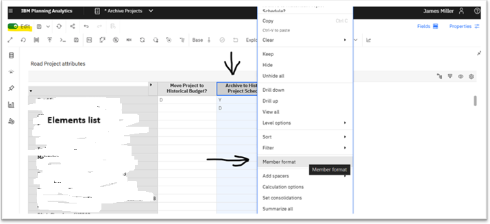
The “Edit <name of selected column> format” dialog will be displayed. There will be three “sections” listed on the left of the dialog: “Format data cells,” “Format header cells” and “Conditional data rules.” Depending upon the data that will be in the cell, you may need to change the data cell format. For example, I have a cell that will display text data and want to add formatting based upon the value of that cell. To do that you need to set the data cell format to “Custom format” (to allow for a text rule to be applied to that cell).
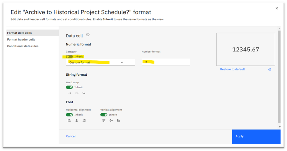
As shown above, I disabled the Inherit property by clicking the toggle to the off position since we do not want this cell to inherit any formatting from the corresponding Planning Analytics cube view. Next, I selected “Custom Format” from the drop-down selector and entered a “#” for the “Number Format” value. Finally Apply was clicked.
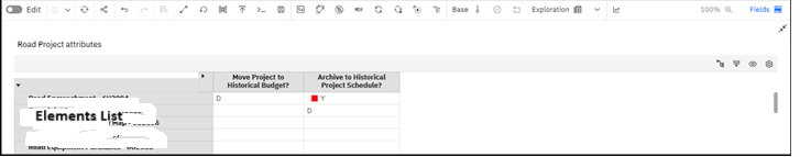
We can skip the “Format header cells” section and go on to “Conditional data rules.” In this section, click Add rule +, then modify the “formatting rule” that was added:
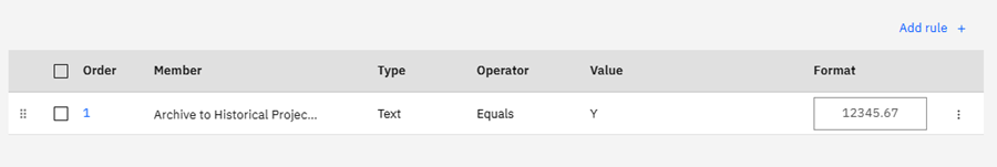
There is an Order value (this is the rule precedence or the order in which the rule will be applied (if there is more than one rule created for this cell), similar to formatting rules in MS Excel. Next, you will see Member. This is the member where I want to attach my rule (you can change the member value if you want or need to by selecting a different value from the drop-down selector). The Type will show as Text (since we formatted the cell in the prior step to a custom format of text) for Operator, I selected “Equals” and for Value I enter a “Y.”
Finally, click on the ellipse icon and then EDIT to add the customize formatting (border color, fill color, font style and color and even add an Indicator):
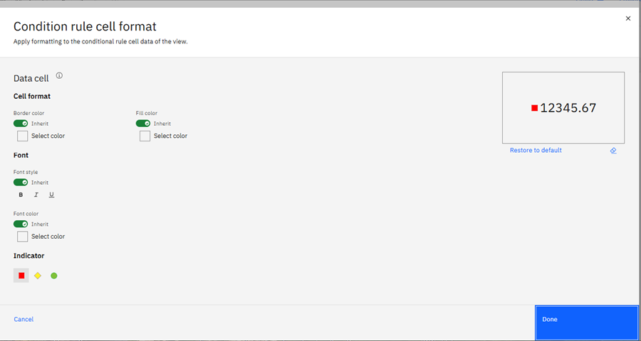
Last step, click DONE then Apply, and refresh your page to view your work!
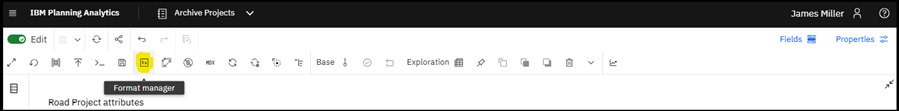
The above (Format member) is a Format Manager shortcut. You can access the full functionality of the Format Manager by clicking the Format Manager icon in the cube view toolbar:
Ask QueBIT
Want some help with using formatting, conditional formatting and using the Format Manger to improve your Planning Analytics Workspace experience? Have a specific question? You can always reach out to QueBIT at support@quebit.com for assistance. We’re here to help!