
Perhaps you work for a residential home builder startup that wants to start using analytics to determine what sort of home they should be building and where. That is, what might be the optimal number of bedrooms, bathrooms and/or square footage for a residential home in each state in the US?
Let’s see how IBM Planning Analytics Workspace (PAW), Powered by TM1, can help!
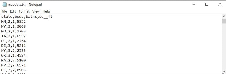
You have some data – a comma-separated values (CSV) file of real-estate transactions by state from last year. In the past you might have started by sharpening your “Excel pencil”, but today, you want to explore the data using PAW, so what do you do?
Step 1. Model your data. Data modeling can be a “deep subject”, but, in a lot of cases, simple is better, so let us use that mind set for this exercise. Ask yourself, what do we want to see? We want to see, for the year, our measures (bedrooms, bathrooms or square footage) by state.
This means that we have 2 “dimensions”. They are “state” (where the home was built) and our “measures” (which contains 3 values: the number of bedrooms in the home, the number of bathrooms in the home and the square footage of the home.
We could stop there, but, since we are pretty sure what we create will be insightful to our business, we most likely will have a new file or data at the end of this year, so let’s add year as a third dimension. Also, since the file is a file of distinct transactions – that is, the data is not intended to be aggregated (like a sum of the total number of bathrooms in all homes, in each state)– we need to provide a transaction ID.
Step 2. Create a Cube. All cubes must have at least two dimensions and we have four, so we are “good” there and can proceed. To create a cube, we first need to create the needed dimensions. There are a number of ways to create dimensions using PAW, with one of the simplest being “drag and drop” which you can read about here.
The Cube Itself
Now assuming you have created the four dimensions, named as “State”, “Home Measures”, “Home ID” and “Year”, we can “snap” them together into a cube.
- Make sure that you are in Edit mode.
- In the Data tree, go to the database where you want to create the cube.
- Expand the database to show the dimensions, cubes, and other associated items.
- Right-click the Cubesgroup, then click Create cube.
- On the Create cubedialog box, type a name for the cube, then in the Available dimensions list, select the dimensions to be included in the cube and then click the right arrow to move the selections to the Cube dimensions list:
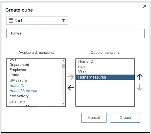
Ready? Sure you are. Now click Create to create the cube.
Step 3. The Data
Our new cube “Homes” is now created so we need to load our file of 2020 home transactions into it. To do that, we will create a TurboIntegrator process that will read the real estate transactions from our file and put them into our homes cube.
Procedure
- Again, in the Data tree, right-click the Processes
- Click Create process.
- Enter a name for the process “Load Home Transactions”.
- Click Create.
Now we have a process, but it does not do anything. So, again in the Data tree, right-click the process and click Edit process.
What should this process do? It should read our file of transactions so in edit mode, click on File and just drag our file on to the process upload area (shown below) and the file name (mapdata.txt) will then appear as selected:
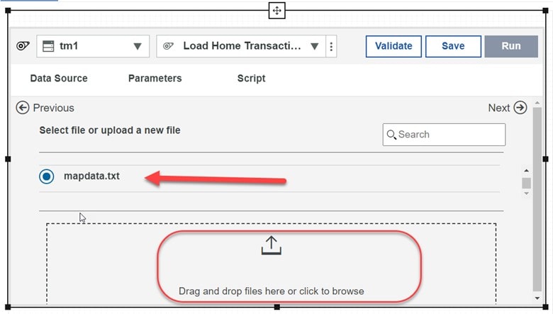
Again, we want to keep things simple, so lets just click on Next (in the upper right).
On the next screen, we want to make just one change. That is, enter a 1 in the Header Records text box (since we know that our mapdata.txt file has a first row that contains columns headings).
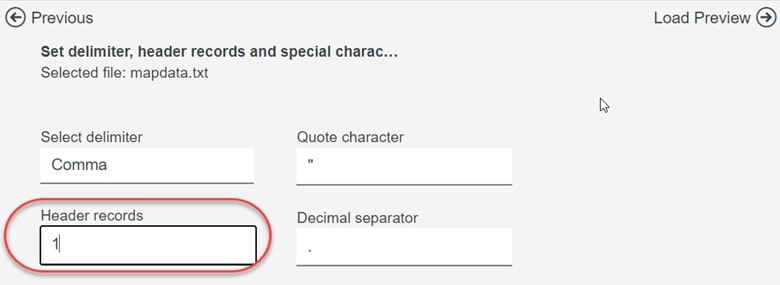
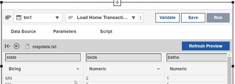
Now click on Load Preview. We should see a preview of our file showing the columns in the file (state, beds, baths and (if you scroll over) sq_ft)
Click on Save. At this point our process will read each transaction (record) in our file and…do nothing else. So, lets click on Script.
Every TurboIntegrator process has four distinct “procedures” that are executed sequentially when you run the process (read about them here). Since we want to load each individual data record into our cube, we can use the CellputN TurboIntegrator function to do that (hint: you’ll need to “cell put” 3 times, one for each measure).
Another thing we need to keep in mind is that we are going to load each file record as a separate, unique “Home ID”, and since these IDs are just random (but unique) numbers, we are going to create a new Home ID for each record “on the fly” as we load the record. We’ll use two other handy functions for that (DimensionElementInsertDirect and DimensionElementComponentAddDirect).
So, here we go:
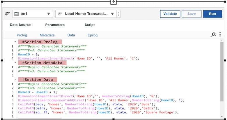
Add the following statement to the #Section Prolog section:
HomeID = 1;
DimensionElementInsertDirect(‘Home ID’, ”, ‘All Homes’, ‘C’);
Add the following statements to the #Section Data section:
HomeID = HomeID + 1;
DimensionElementInsertDirect(‘Home ID’,”, NumberToString(HomeID), ‘N’);
DimensionElementComponentAddDirect(‘Home ID’, ‘All Homes’,NumberToString(HomeID), 1);
CellPutN(beds, ‘Homes’, NumberToString(HomeID), state, ‘2020’,’Beds’);
CellPutN(baths, ‘Homes’, NumberToString(HomeID), state, ‘2020’,’Baths’);
CellPutN(sq__ft, ‘Homes’, NumberToString(HomeID), state, ‘2020’,’Square Footage’);
Note: do not insert any of your statements between the “generated statements” start and finish lines, as anything between these lines can be overwritten.
Finally, click Save to save the updates to the process. If you don’t have any typos in what you typed, you can now click on Run. The process will run, read your file and load the Homes cube.
Step 4. Map it
Since we wanted to visualize our data (rather than look at rows and columns in a report) we can utilize a map visualization to show patterns in our data by geography (state, in our case).
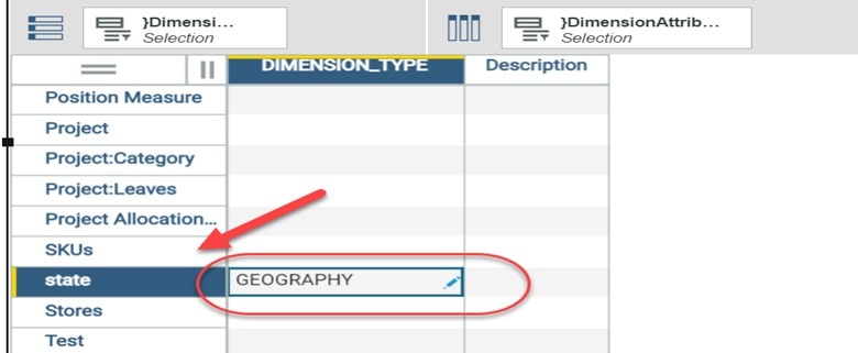
Before we can create our map, we need to do one more thing and that is to make sure that PAW “knows” that our state dimension is “designated” as a geography “dimension type”. This is a dimension attribute in the }DimensionAttributes control cube. This is set at the intersection of the dimension that you want to define as a geography dimension (state) and the DIMENSION_TYPE attribute, by entering “Geography”:
Okay, now we can:
- Create a view in PAW from our Homes cube with the rows displaying the designated geography dimension (state).
- Set the visualization type to be a Legacy Map.
- Make sure the map fields are set with Regions Heat: Baths and Filters of All homes and All Years. The resulting display will appear as a scrollable and zoomable map visualization:
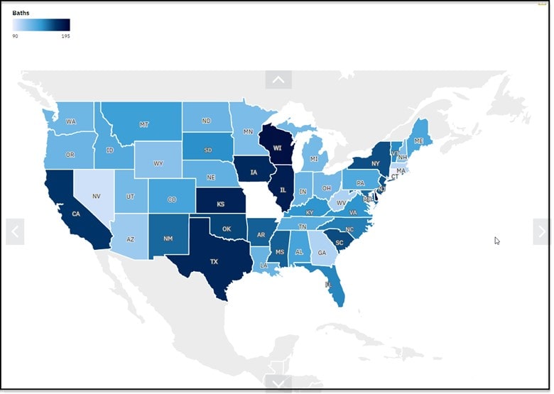
Seems like the homes with the most bathrooms were built in CA and Tx!
Of course, what we did here is just a simple “proof of concept” exercise, but it literally took only a few minutes. IBM Planning Analytics is full of fun features and functionality. Not sure what to do next? Check out the ask QueBIT’s knowledgebase or give us a call!
The content of this article was developed using IBM Planning Analytics Workspace 2.0.60 running on the IBM Cloud.