
IBM defines a cube as “…the basic container for data…” and a cube view as “…the definition of how a cube’s dimensions are arranged…”. Planning Analytics cubes can each have multiple views defined and typically, each cube will have specific views designed to assist with common reporting needs.
Common Views
In addition to defining various common views, it is always a good idea to also define a default view for each cube in a model. A default view is the view that will be loaded if you just double-click the cube or open the cube without first selecting one of the specific saved views.
You can save any view of cube data for quick access in the future and any view as the cubes default view. Remember though that each cube view must have a unique name and a cube can have only one (actually one public and one private) default view. Default views automatically display in the Cube Viewer or when you double-click the cube name in the Server Explorer window.
When you create a common view, the intention is to arrange the dimensionality and data of the cube in a way that you need to view the data so that you don’t have to take the time to re-arrange the dimensions and data each time you need to view the data in a certain way. For example, you might define a balance sheet view, or an income statement view for a Finance cube. You can read about how to create a new cube view here.
Default Views
When you create a default view, the objective is a bit different, that is you want to arrange the dimensionality and data in such a way that the view loads as quickly as possible. This is typically done by selecting only aggregated elements for each dimension, such as “Total Company” or “All Regions” (rather than listing all of the company or region elements). When a cube view loads, the more elements that are visible, the longer it will take to load. Typically, setting each dimension to the “top level” element (aggregation) will improve the view load time, however, there is a nuance in that sometimes this “Top of the House” (e.g., Total Regions etc.) selection will be slow if it is at the top of a very large dimension and has to consolidate or “rollup” up MANY rule-calculated values. In this case, it is better to select a default as one of the “smaller” elements in the dimension.
Leveraging MDX Expressions
Once you have a view defined you may want to take things a bit further and make the view dynamic by using a dynamic subset within the view. A dynamic subset can use an MDX expression to automatically filter elements from a dimension (rather than showing a static list of pre-selected elements). For example, you could define a static subset on a Year dimension to show the current “Reporting Year” and then manually update the subset as part of a reporting year-end process or, you could use an MDX expression to drive or change the subset automatically so that it always shows whatever the current reporting year is without anyone having to update it – a much more efficient approach.
Use Case
For illustration, here is a simple (but practical) use case using the “Planning Sample” Planning Analytics (PA) server that is included with the PA installation. In this server there is a cube named “plan_Report”. Let’s suppose that this cube is used for monthly reporting. Here is the cube and its dimensionality (shown in the TM1 Architect user interface):
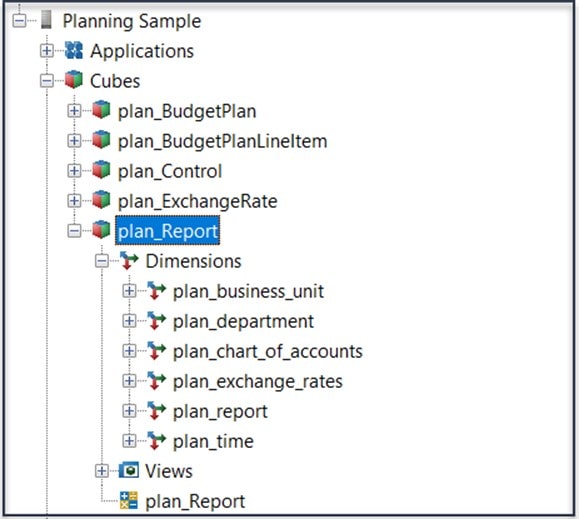
There are already a number of views defined for this cube, but let’s create a default view that will load a fast as possible when a user opens the cube. To do that you can:
- Double-click the cube name
- Modify the view to meet our requirements. For this default view we want to select the highest-level aggregated element for each dimension:
- plan_business_unit = “Total Business Unit”
- plan_department = “Total Organization”
- plan_chart_of_Accounts = “Net Operating Income”
- plan_exchange_rates = “local”
- plan_report = “actual”
- plan_time = “2005”
We’ll also “drag” the plan_chart_of_accounts dimension down as the rows dimension and “drop” the plan_time dimension as the columns in the view. Next click Actions > Save as and Default (to save the view as the default view for the cube):
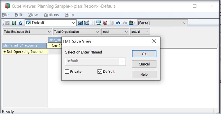
Now we have an efficient default view defined for the cube, since all of the dimensions are set to their highest level of aggregation. No matter how many elements are added to each of the dimensions or how many additional periods are added to the plan_time dimension, our default view will always load very quickly.
Reporting Year
The only problem with this view is that as the Reporting Year changes, an administrator will need to open the default view, change the selected plan_time element (to the current Reporting Year) and re-save the view (as the updated default). With everything else an administrator may need to do, this is one task they shouldn’t need to deal with, so you can alter the default view to use an MDX based, dynamic subset that always selects the current Reporting Year automatically.
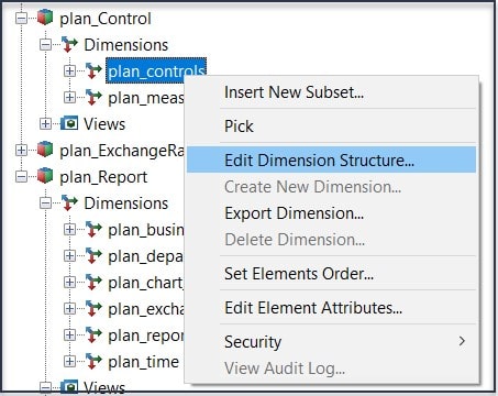
There is a “global settings” cube within the server named “plan_Control”. This cube contains values that “control” all planning processes and reports. This cube already has the values: “Data Source” and “Corporate Currency”, so why not add a new value to control the current Reporting Year? To do that:
- As an administrator, right-click on the “plan_controls” dimension and select Edit Dimension Structure…
- In the Dimension Editor, select Edit then Insert Element. On the Dimension Element Insert dialog, you can enter “Reporting Year” as the Insert Element Name, leave “Simple” as the Element Type and 0.0 as the Element Weight. Then click Add and to finish, OK:

While we are here, let’s repeat this step and add another element named “Prior Reporting Year”. After adding these new elements, if we open the plan_Control cube, we can enter the values for the elements we just added:
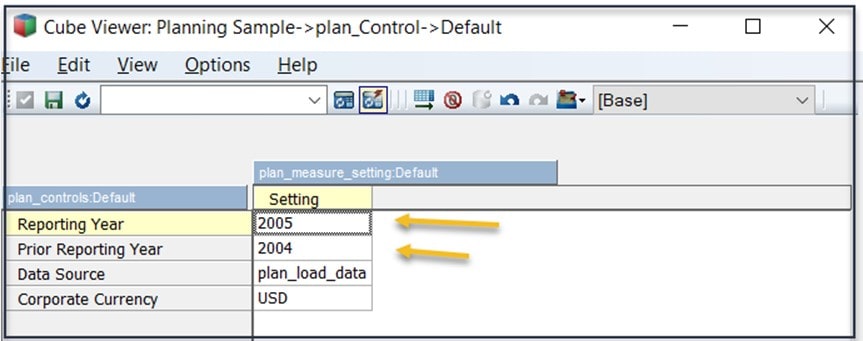
You might think that the current Reporting Year value in the plan_Control cube still needs to be maintained, but the difference from manually updating the subset is that all views, reports and processes can now leverage the plan_control cube to determine the current Reporting Year – so when you change it once here (in the cube) everything is up to date and “in sync” (you could also implement a rule or process that would maintain the Reporting Year values in the plan_Control cube to further automate the process).
Add the MDX
To leverage these plan_Control cube values, we’ll create a simple MDX driven subset on the plan_Time dimension:
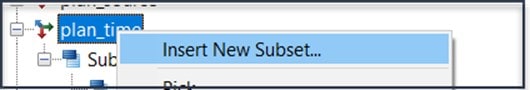
- As an administrator, right click on the plan_Time dimension and select “Insert New Subset…”:
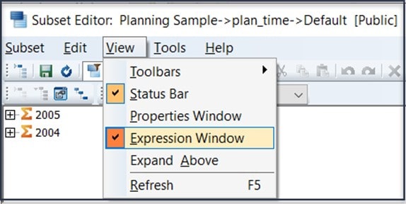
- Within the Subset Editor, select View then Expression Window.
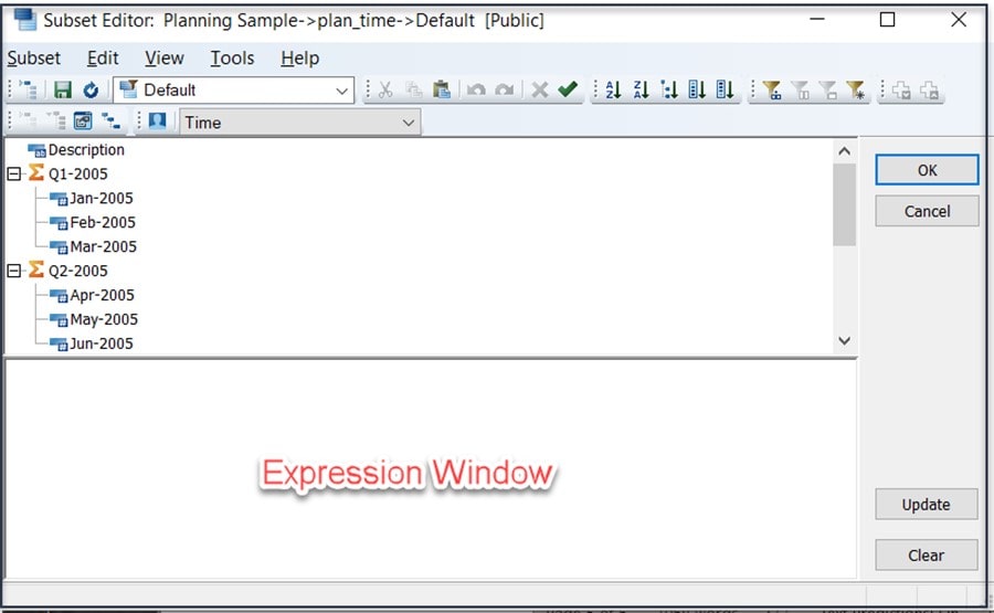
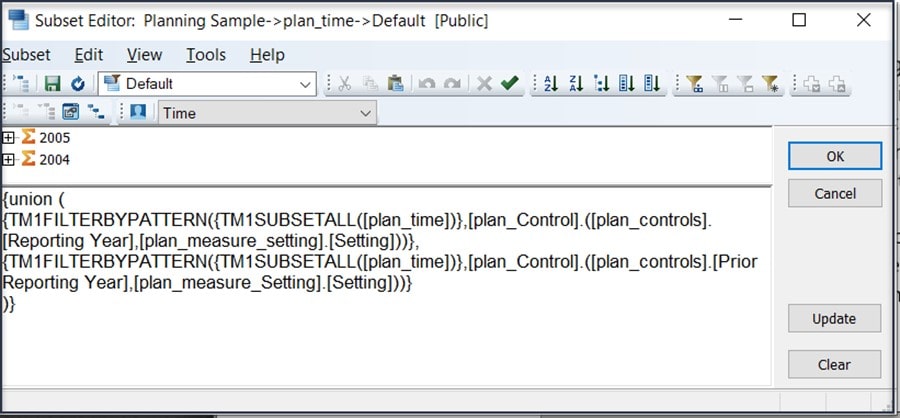
You should now see the Subset Editor with the “Expression Window” displayed across the bottom of the dialog:
The expression window is where you can add the MDX statement that will maintain the subset. To build this MDX expression, you can use three common MDX functions: TM1SUBSETALL which returns a PA/TM1 subset containing “All” elements of a dimension, TM1FILTERBYPATTERN which returns all the elements that are members in a “set” with names matching a pattern and UNION which returns a set generated by the union (or the combination) of a one or more sets. The statement will look like this:
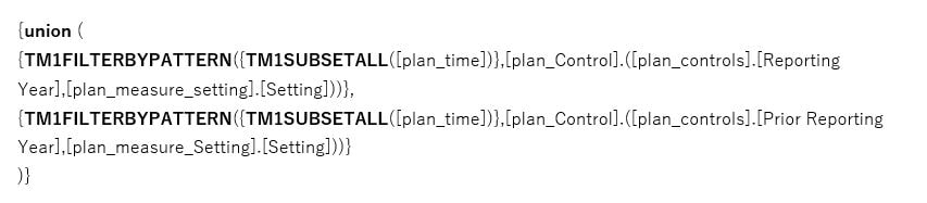
Although how these functions work is probably not too hard to conceptualize, adding the syntax to the overall expression does make it confusing (i.e., the “{“ and “(“ characters). It sometimes helps to break the expression down, so notice where the expression uses the dimension name “plan_time” and the cube name “plan_Control” as well as the explicit mentioning of the plan_Control cube dimensions (“plan_controls” and “plan_measure_setting”). Altogether, this expression “queries” the cube values of “Reporting Year” and “Prior Reporting Year” and loads those values into the subset (assuming they exist in the dimension).
- Once you enter the full MDX expression, click “Update”, you can then select Subset and Reload to execute the expression. If you have values entered in the plan_Control cube, and they exist in the plan_time dimension, you should see the following (make sure you save the updated subset before you close the Subset Editor by using Save As… and providing a unique name):
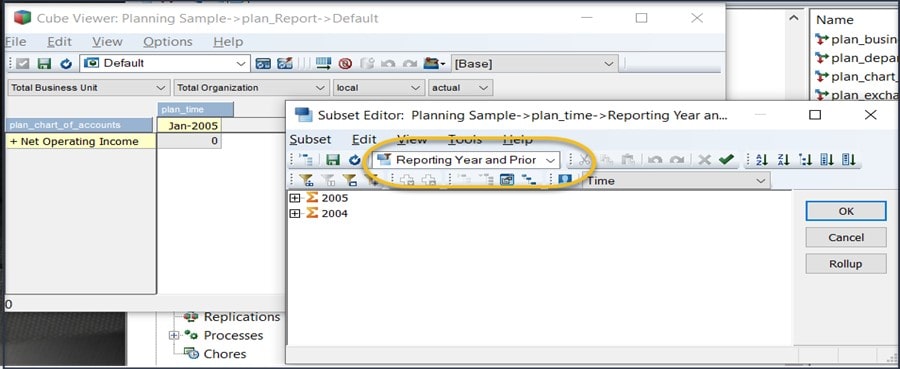
Now the subset will always reflect the (Reporting Year and Prior Reporting Year) values in the plan_Control cube. The final step in this process is to update the default view for the plan_Report cube so that it uses this dynamic subset. To do that, you simply open the default view, select the plan_time dimension and select the subset name (I named it “Reporting Year and Prior”) and then click OK.
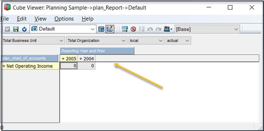
The default view will now reflect the Reporting Year and the Prior Reporting Year. Re-save the default view and the view will always be up to date:
This MDX utilized values from a cube (the plan_control cube) and we were able to type it directly into the Expression Window. Another method for creating an MDX is by using the Marco recorder. You can read about that approach (and more about MDX) here.
Interested in Learning More?
Are you interested in exploring more simple tricks to make Planning Analytics more user friendly? Then Contact QueBIT today and we’ll be happy to help you take advantage of all of the features of Planning Analytics. This article utilized PAW version 2.0.70.59, want help upgrading your PAW? QueBIT can help with that too. Like this post? Feel free to connect with me on: LinkedIn.